Telescope Eyepiece Pricing

If you are a newbie astronomer like me, you may be confused by the variety and pricing of eyepieces available.

I used information from the Orion Holiday 2017 catalog on individually sold eyepieces, including the apparent field of view (AFoV from 52 to 106 degrees), diameter (1.25" and 2“), and length (2.5 to 42 mm) to predict the price ($30-$830, in US dollars).

library(tidyverse)

EP <- read.csv("EyePieces.csv") %>%
  mutate(
    fDiam = as.factor(Diameter)
  )

DT::datatable(
  EP[, c("Make", "Model", "AFoV", "Diameter", "Length", "Price")],
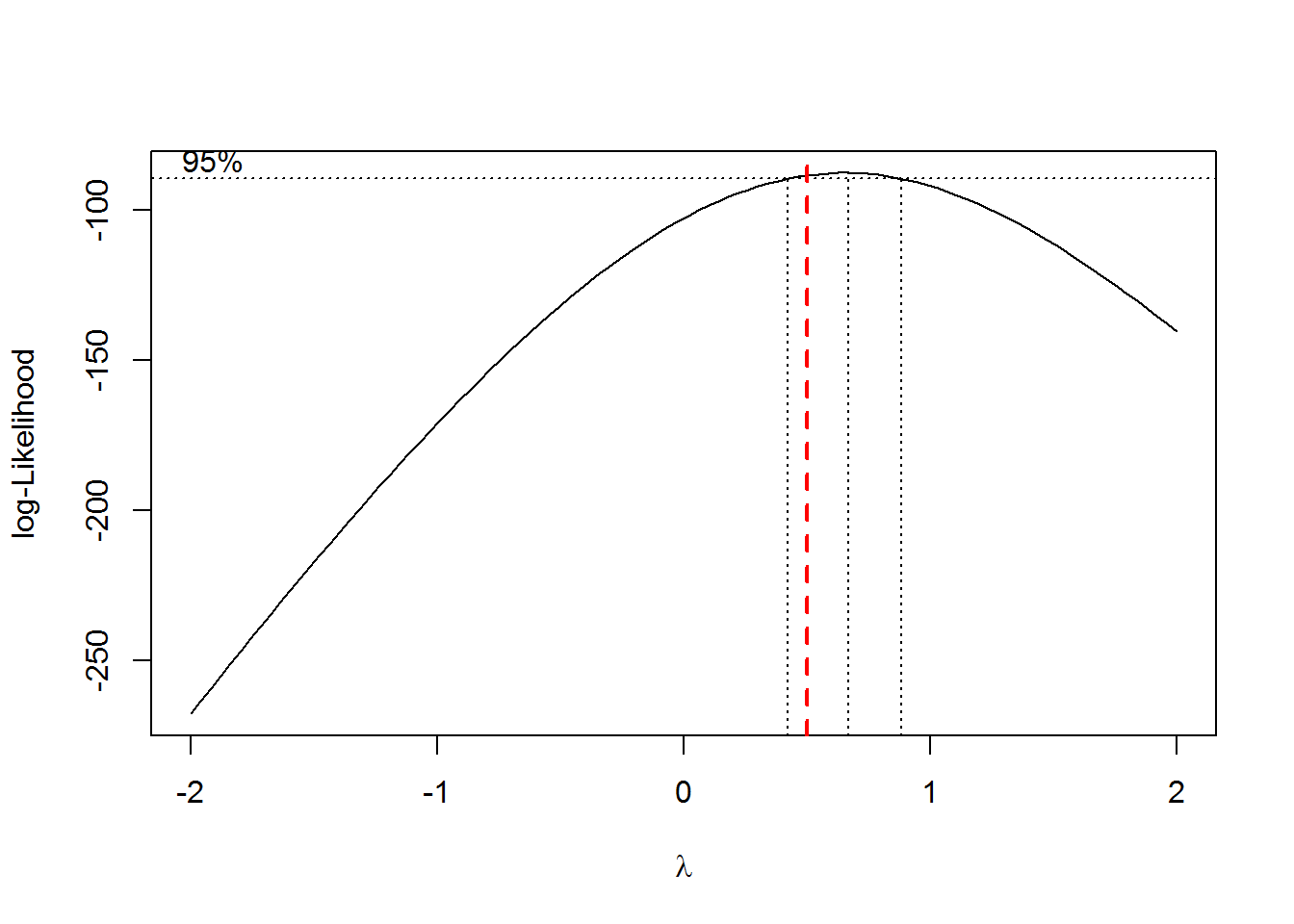
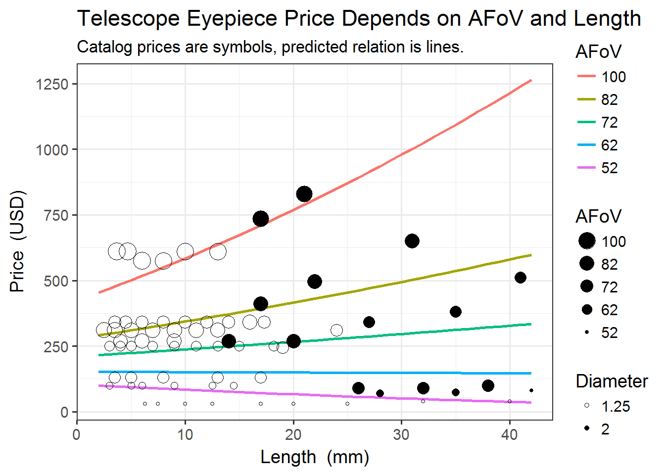
  options=list(pageLength=5))

What factors contribute to the pricing? I fit a model predicting price from the three metrics available on all eyepieces (and all two-way interactions). A square root was suggested for the response (Box-Cox transformation). Apparent field of view was the strongest predictor of eyepiece price, with length (and its interaction with AFoV) also contributing.

EP %>%
  glm(Price ~ (AFoV + Length + fDiam)^2, data=.) %>%
  MASS::boxcox()
abline(v=0.5, col="red", lty=2, lwd=2)

fit <- step(
  glm(sqrt(Price) ~ (AFoV + Length + fDiam)^2, data=EP), trace=0)
summary(fit)$coef

##                 Estimate  Std. Error    t value     Pr(>|t|)
## (Intercept) -1.131293845 2.820420698 -0.4011082 6.895981e-01
## AFoV         0.217372305 0.038755751  5.6087754 4.045853e-07
## Length      -0.596128425 0.176439168 -3.3786626 1.209211e-03
## AFoV:Length  0.009523264 0.002636975  3.6114350 5.779988e-04

PopularAFoV <- c(52, 62, 72, 82, 100)

Predplot <- expand.grid(AFoV=PopularAFoV, Length=2:42) %>%
  mutate(
    Predicted = predict(fit, newdata=.)^2,
    fAFoV = factor(AFoV, levels=rev(sort(unique(AFoV))))
  )

ggplot(EP, aes(Length, Price)) +
  geom_line(map=aes(Length, Predicted, color=fAFoV, group=fAFoV), 
    size=1, data=Predplot) +
  scale_color_discrete(name="AFoV") +
  geom_point(aes(shape=fDiam, size=sqrt(AFoV))) +
  scale_shape_manual(values=c(1, 16), name="Diameter") +
  scale_size_continuous(name="AFoV", breaks=rev(sqrt(PopularAFoV)), 
    labels=rev(PopularAFoV)) +
  labs(x="Length  (mm)", y="Price  (USD)",
    title="Telescope Eyepiece Price Depends on AFoV and Length",  
    subtitle=
      "Catalog prices are symbols, predicted relation is lines.") +
  theme_bw(base_size=14)

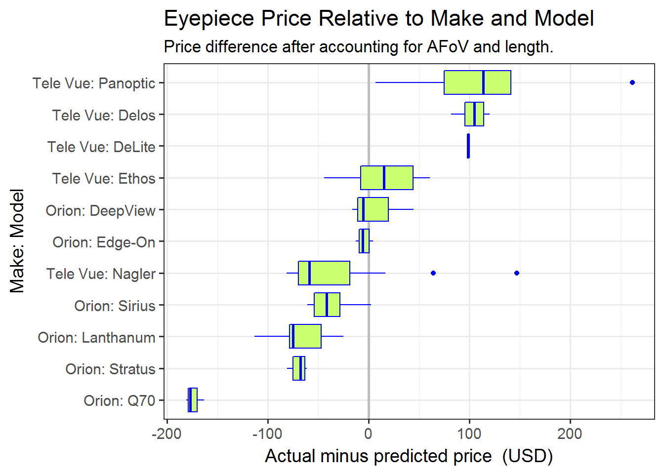
I was curious if and how the make and model of the eyepieces contributed to the prices. So, I calculated the difference between the actual price and the predicted price.

EP.pred <- EP %>%
  mutate(
    Predicted = fit$fitted.values^2,
    Pricediff = Price - Predicted,
    BM = paste0(Make, ": ", Model)
  )

EP.mean <- EP.pred %>%
  group_by(BM) %>%
  summarise(mean=mean(Pricediff)) %>%
  arrange(mean)

EP.BM <- EP.pred %>%
  mutate(
    BM = factor(BM, levels=EP.mean$BM)
  )

ggplot(EP.BM, aes(BM, Pricediff)) +
  geom_hline(yintercept=0, size=1, color="gray") +
  geom_boxplot(fill="darkolivegreen1", color="blue") +
  coord_flip() +
  labs(y="Actual minus predicted price  (USD)", x="Make: Model",
    title="Eyepiece Price Relative to Make and Model",
    subtitle="Price difference after accounting for AFoV and length.") +
  theme_bw(base_size=14)

Most of the Tele Vue models are priced higher than predicted, and most of the Orion models are priced lower than predicted. Reading the descriptions in the catalog, it’s not obvious to me what is contributing to these differences.